
Emergent Populations Derived With Unsupervised Learning of Human Whole Genomes
A republish of a hidden paper where I describe my invention of a Large Genome Model (LGM).

Context and Historical Significance:
A Large Genome Model (LGM) is a type of foundational AI that reads a large corpus of DNA code (i.e., ATGC) and tells humans what this code means. Such an AI can tell us about the meaning of life, where people from different heritages came from thousands of years ago, as well as how to make medicines to cure ~10,000 rare genetic diseases.
I published the LGM described below in (Njie BioRxiv 2018). This therefore is the first LGM in existence. I’m the flag-bearing inventor of LGMs. 🌟🇬🇲.
This LGM is old by AI standards (no transformers, etc), but still outperforms 23andMe today. In small circles, LGMs are expected to leapfrog AlphaFold for the next most valuable technology because they can help us make new medicines.
I am the founder of a company called Ecotone. We are specialize in building custom LGMs from the ground up to help us end genetic diseases.
For more deets on why LGMs are so valuable (scientific and commercial landscape, etc), it’s innovativeness, as well as the human story behind the build (spoiler; there was rejection, perseverance, and drama including being forced to withdraw the paper), see the accompanying article The value and drama of the first Large Genome Model. It’s written in non-technical language so the story is accessible to those of you that are not knee-deep in the fields of AI and genetics.
Thank you for reading, and please show your support by subscribing and sharing! I’m available for questions and investment opportunities emalick@ecotone.ai
Abstract:
Artificial intelligence (AI) holds great promise to precisely classify human ancestry and the genetic causes of complex diseases. I have constructed an unsupervised machine learning paradigm that examines the whole genome as a hyper-dense, nonlinear, multidimensional feature space. The AI system culminates in 26 neural network neurons each sensitive to a specific heritage that can identify an individual’s component genetic heritages with a top-5 error of <0.5%. Importantly, I observed some populations previously thought to belong to single stratum are composed of multiple strata – for instance Japan is defined as a uniform population using previous methods. I found that the Japanese individuals segregate to two very distinct populations. This work represents an essential step towards understanding the genetic background of patients to enable precision medicine causal disease gene identification.
Introduction:
Ancestry classification is a central problem in human genomics. In precision medicine where one identifies the genetic causes of disease, it is important to control for population difference effects since true disease-causing mutations can be masked by subtle differences in genetic ancestry between patient and control groups (Kaplanis, et al., 2018; Tian, et al., 2008). Ancestry classification is also widely used to help people better understand their family history and identity (Hellenthal, et al., 2014). However, existing methods for genetic ancestry inference are limited by the power of the statistical methods employed to analyze the data.
Recent advances in machine learning and artificial intelligence (AI), in particular non-linear dimensional reduction and neural networks, hold promise for the analysis of large and complex datasets such as WGS (Haasl, et al., 2013; Kaul, et al., 2017; Omberg, et al., 2012; Romero, et al., 2017). Dimensional reduction methods aim to transform high dimensional datasets (e.g., billions of base pairs) into a low dimensional representation (e.g., 2D or 3D plot) for easy visualization, while ideally preserving data structure. However, traditional linear methods such as principal component analysis (PCA) (Jolliffe, 2002) and classical multidimensional scaling (MDS) (Torgerson, 1952) struggle when faced with complex and non-linear datasets such as genomic data. Recently, the unsupervised machine learning technique t-SNE (van der Maaten and Hinton, 2008) was developed for non-linear dimensional reduction. t-SNE aims to minimize the Kulback-Leibler divergence between a Gaussian distribution of the original high dimensional data and a Cauchy distribution of the low dimensional representation by applying gradient descent, which helps to preserve the local structure of the data while revealing global structures in the form of clusters (van der Maaten and Hinton, 2008). t-SNE consistently outperforms (van der Maaten and Hinton, 2008) other non-linear dimensional reduction methods such as Sammon mapping (Sammon, 1969), Isomap (Tenenbaum, et al., 2000), and locally linear embedding (Roweis and Saul, 2000).
As with non-linear dimensional reduction techniques, neural networks have recently seen considerable advances in scale and complexity and are routinely employed today in image and sound recognition (He, et al., 2015; Krizhevsky, et al., 2012; Sabour, et al., 2017; Szegedy, et al., 2015). Neural networks are composed of linear algebraic hyperplanes (i.e., neurons) that preserve localized information in receptive fields. They are inspired by biological neurons in the brain and are ideally suited to complex classification tasks such as genetic population stratification (Bridges, et al., 2011).
Here I present a novel method combining t-SNE-based non-linear dimensional reduction followed by a neural network that learns the re-imagined t-SNE space as a novel cartographic genetic features map to accurately dissect an individual’s genetic ancestry. I found populations previously thought to be uniform are surprising segregated into more complex strata. To my knowledge, this report is the first to explore the combination of t-SNE with a neural network for ancestry classification and analysis. This approach is broadly applicable to other whole genome datasets and is a powerful tool for the study of both genetic ancestry and diseases.
Results:
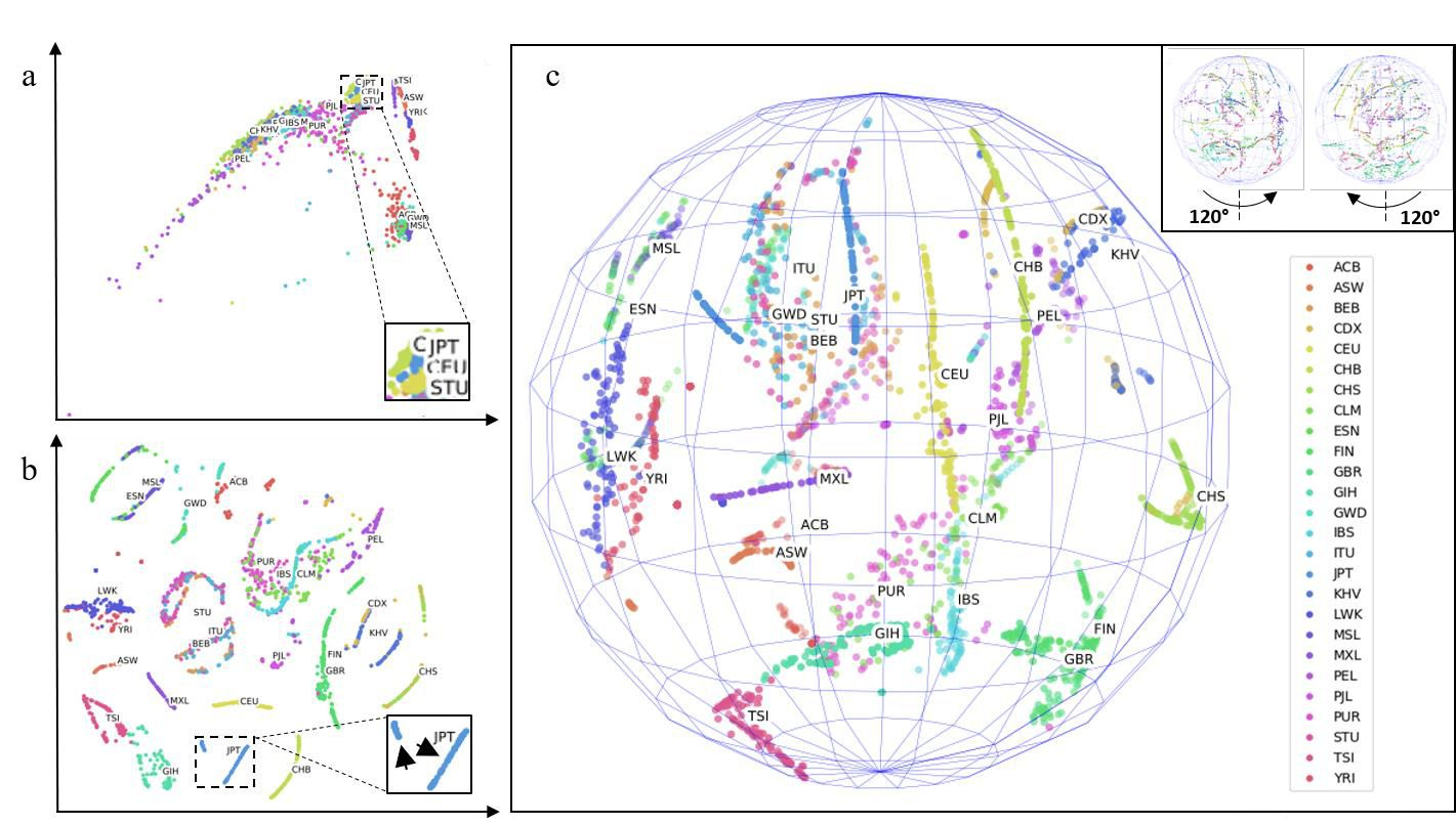
Figure 1. Genetic maps of the 26 world populations sampled by the 1000 Genomes Project. (A) 2D PCA. (B) 2D t-SNE. (C) 3D t-SNE. Insets in (A) and (B) are centered on JPT. Note JPT is stratified to distinguishable small and large component populations (arrowheads within inset in B). Inset in (C) shows views rotated +-120 degrees. Two outlier points were excluded in (C). Labels were not part of input training data (unsupervised training); rather, labels were applied post-hoc for visualization of cluster accuracy. See Methods for full descriptions of 3-letter heritage abbreviations.
The 1000 Genomes project is an international consortium initiated in 2008 to sequence whole genomes from willing donors worldwide. The third and final phase of the project resulted in a publicly accessible repository of thousands of individuals. I performed analyses on chromosome 1 of these genomes - extracting a hyper-dense map of ~6 million SNPs for each individual. I then inputted these SNPs into KING to obtain pairwise coefficients of the relatedness of each individual to every member of the set (see Methods). The KING map is a high-level feature space composed of thousands of dimensions that are impossible to interpret with human eyes. I therefore addressed this with the unsupervised machine learning dimensional reduction technique t-SNE. My results indicate clear clustering and separation of clusters where each point within a cluster is a hyper-deep abstraction of ~6 million SNPs (Figure 1, labels added post-hoc and were unknown during cluster separation, see Methods for full descriptions of 3-letter heritage abbreviations). Compared to 2D PCA, which does not produce clear clusters (Figure 1A), my t- SNE results provide a clear visualization of clustering and separation of individuals according to their heritages (Figure 1B and 1C, dynamic cluster movement in Figure S1 movie). This direct observation of cluster separation validates the effectiveness of my non-linear dimensionality reduction approach. In 3D t-SNE, the clusters are distributed in the shape of a sphere (Figure 1C), which provided further separation of clusters than in 2D t-SNE (Figure 1B). Further dimensional increases (e.g., 4D – 6D) were explored. These separations cannot be presented visually. However I present in later paragraphs evidence of their utility.
Note that in 2D as well as 3D, some populations previously thought to be segregated are singular and conversely, some populations thought to be singular are surprisingly stratified into multiple populations. For instance, JPT (Japan) clearly is composed of two populations (Figure 1B, inset arrowheads). Japan has at least three minority groups: the Ryukyuan of Okinawa, the Yamato which are thought to have Japanese and Korean ancestry and the Ainu which are the original inhabitants of the Japanese peninsular. I hypothesize that the minor Japanese cluster is composed of one or more of these populations. To my knowledge, this data is the first de novo separation of Japanese individuals into multiple strata using purely whole genome data.
Though t-SNE performed well in segregating populations, it is a visualization algorithm with no power to perform classification. I therefore considered the t-SNE space itself as a feature space. Traditionally in machine learning, t-SNE is used post-hoc to analyze the activations of neurons within neural nets to see how they learned (Olah, 2015). I used an inverse approach, i.e., the t- SNE space is a set of Cartesian coordinates representing human genetic features map. Therefore, coordinates are treated similar to longitude and latitude pairs on a map of Earth representing regions such as Gambia (GWD), Finland (FIN), and so forth. Each coordinate is a representation (as evidenced by clustering) of a dimensional space of KING values in the thousands and before it, SNPs in the millions, and prior to that, the adjacent DNA bases these SNPs represent, which number in the billions.
Therefore, the Cartesian coordinates are useful, simplified abstraction of the high dimensionality of complex data and are therefore ideal candidates for neural net classification. I thus constructed a 5-layer neural net to accept the t-SNE-transformed WGS data of the individuals in the 1000 Genomes Project set (see Materials and Methods). The output of my neural net was 26 neurons, each sensitive to one of the 1000 Genomes Project heritages.
Histograms of these firings indicate that each neuron is highly sensitive to a particular heritage (Figure 2A and 2B). For some particular individuals, one neuron may fire at about 95% capacity while the sum of all the other neurons is about 5%, with most not firing at all (Figure 2A). This pattern indicates that the neural net is confident in assigning a particular heritage to the individual. For many individuals, several neurons fire simultaneously, indicating multiple heritages, which I interpret as the neural net being less confident in assigning a particular heritage to an individual (Figure 2B). Reasons for this uncertainty could be that the individual in question is extensively admixed or that the primary heritage of the individual differs from what was self-reported.
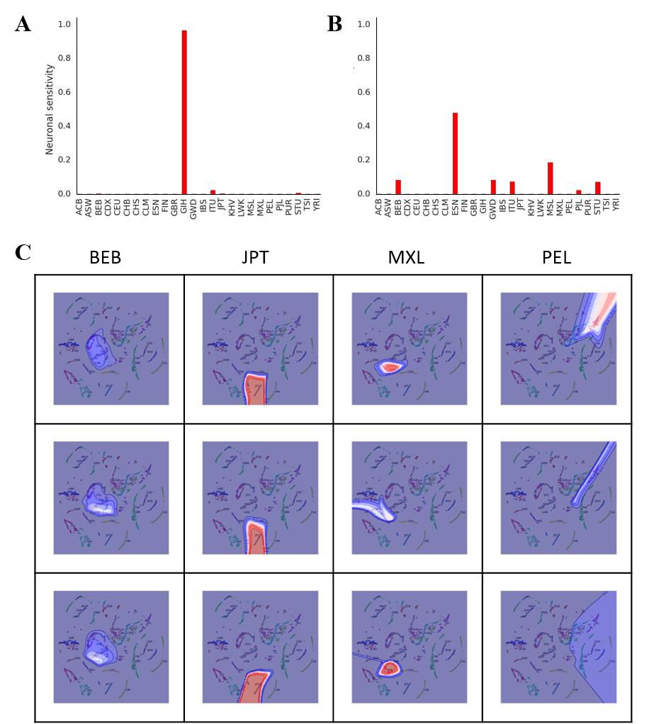
Figure 2. Neural net representation of an individual’s heritage. (A), (B) Heritage-based output neuron firing for two representative individuals using 3D t-SNE. (C) Contour plot of neural net activations.
Contour lines were plotted in 0.1 intervals from 0 to 1, and colored according to the ‘seismic’ colormap in Matplotlib (i.e. 0 = Blue, 0.5 = White, 1.0 = Red). Each contour plot is specific for a single output neuron heritage (indicated by the column labels) and overlaid on the 2D t-SNE plot for visualization. Rows represent three separate runs of the neural net.
To provide mechanistic insight into how the neural net is performing its classification, I generated a similar neural net as my nolearn/Lasagne/Theano stack using Scikit-learn. This enabled me to construct contour plots of neuronal activations to directly observe spatial receptive fields of output neurons (Figure 2C). These were overlaid onto 2D t-SNE plots for easy visualization. My results show that for some heritages (e.g., JPT), the contour lines are close to each other and the corresponding output neuron fires at or close to 1, indicating detection of a tight cluster and highly confident classification by the neural net. Moreover, the contour pattern remains similar across multiple runs and envelops the JPT cluster in 2D t-SNE space, indicating highly reproducible and accurate classification by the net. For MXL, the neural net mostly performs classification well, but is less confident than as with JPT. This is shown by the fact that in one of the three runs, the maximum activation of the MXL neuron was ~50% compared to the other two runs, and the contour lines do not form a tight cluster. However, for the other two heritages tested (e.g. BEB and PEL), the neural net displays uncertainty in its classification (i.e., the contour shapes do not match across multiple runs). This result could be explained by the fact that these heritages closely neighbor or overlap other clusters in t-SNE space. Since the neural net is trained on t-SNE coordinates, close neighbors or overlapping clusters could cause uncertainties in the neural net classification.
Next, I tested how different dimensions of t-SNE affected the performance of my neural net classification (Figure 3). To estimate the accuracy of the neural net, I adopted Top-n error scores traditionally used in the machine learning community. Top-1 error is the likelihood that the ground truth label is not the top label predicted by the neural net (e.g., the individual claims to be Yoruba but the net’s top firing neuron is not Yoruba). My results show that 4D t-SNE allowed for the best neural net performance (lowest top-1 error of ~15%). However, further increases of the number of dimensions resulted in a drop in neural net classification performance, i.e., top-1 error of ~20% and ~68% for 5D and 6D t-SNE, respectively (Figure 3A). Confusion matrices of 2D through 6D t-SNE show that the neural net generally predicts these 26 labels well, with 4D t- SNE giving the best performance (Figure 3B). I believe the false predictions here are due primarily to misreporting of heritages and secondarily to possible overlap of clusters in t-SNE space (see Discussion section for more details). Additionally, although 5D t-SNE is the second- best performer ahead of 3D t-SNE from a top-1 error perspective, it suffers from poor overfitting (Figure 3C).
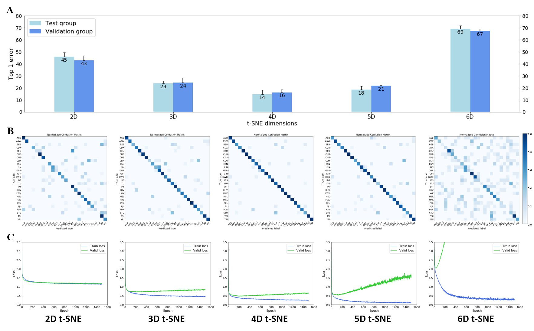
Figure 3. Performance of the neural net heritage classification from 2D to 6D t-SNE. (A) Top-1 error for 2D – 6D t-SNE. Bars represent the average of n = 3 passes of testing sets in the neural net; each testing set is randomized and contains 375 individuals. Error bars represent standard deviation. (B) Confusion matrices for 2D – 6D t-SNE. 26 x 26 confusion matrices were plotted after normalization. (C) Loss function of neural net across 2D – 6D t-SNE. Training (blue) and validation (green) curves were plotted for 2D to 6D t-SNE.
In order to further improve the accuracy of my neural net classification, I drew inspiration from the classic concept of data augmentation, which seeks to augment a training dataset using image translations, reflections and rotations etc. so as to take into account important spatial relationships or hierarchies between objects (Figure 4A) (Krizhevsky, et al., 2012). Instead of using these classic transformations, I experimented with the t-SNE parameter of perplexity to generate different frames containing different representations of the data, which I could use for data augmentation. I named this technique superposition as the neural net is forced to find coherence of identical input data that are in different states. My results show that low perplexity (=1) results in no clusters while high perplexity (=1000) results in cluster collapse (Figure 4B), not unlike the PCA output (Figure 1A). I decided to utilize the frames generated by perplexity = 30 and 40 as superposition inputs for the neural net because they represent a good middle ground that retains clustering while varying cluster positions slightly.
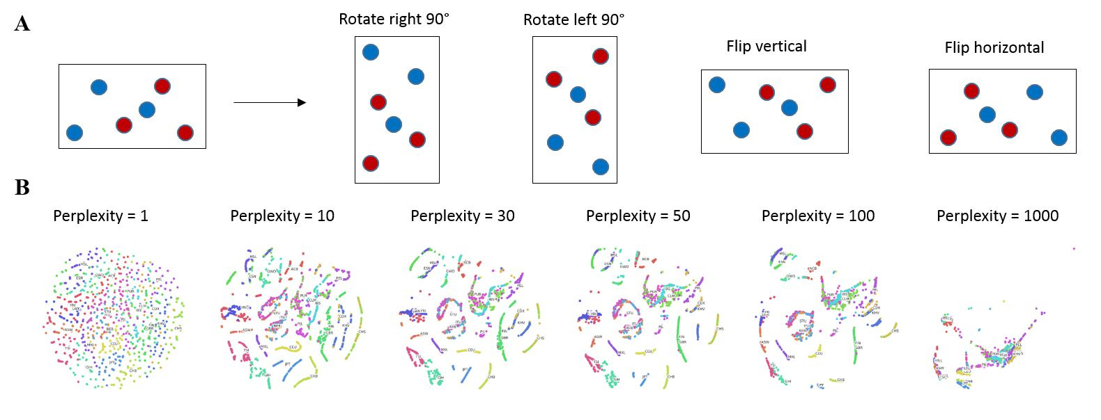
Figure 4. Data augmentation by superposition. (A) Classic data augmentation techniques. (B) Effect of perplexity on 2D t-SNE output.
To study the effect of superposition on neural net accuracy, I compared the top-1 to top-5 error scores for 2D to 6D t-SNE, both with and without superposition. Top-5 error is the likelihood that the correct label is not within the top five labels predicted by the neural net (e.g., the individual claims to be Yoruba, but the neural net’s top five predictions do not include Yoruba). My results indicate that the top error scores decrease significantly across all dimensions for both test and validation groups. Of note, superposition had the greatest impact on improving the accuracy of the neural net at low dimensions (2D t-SNE), decreasing top-1 and top-2 errors from ~45% to ~25% and ~25% to ~8% respectively (Figure 5). At higher dimensions, the effect of superposition was marginal.
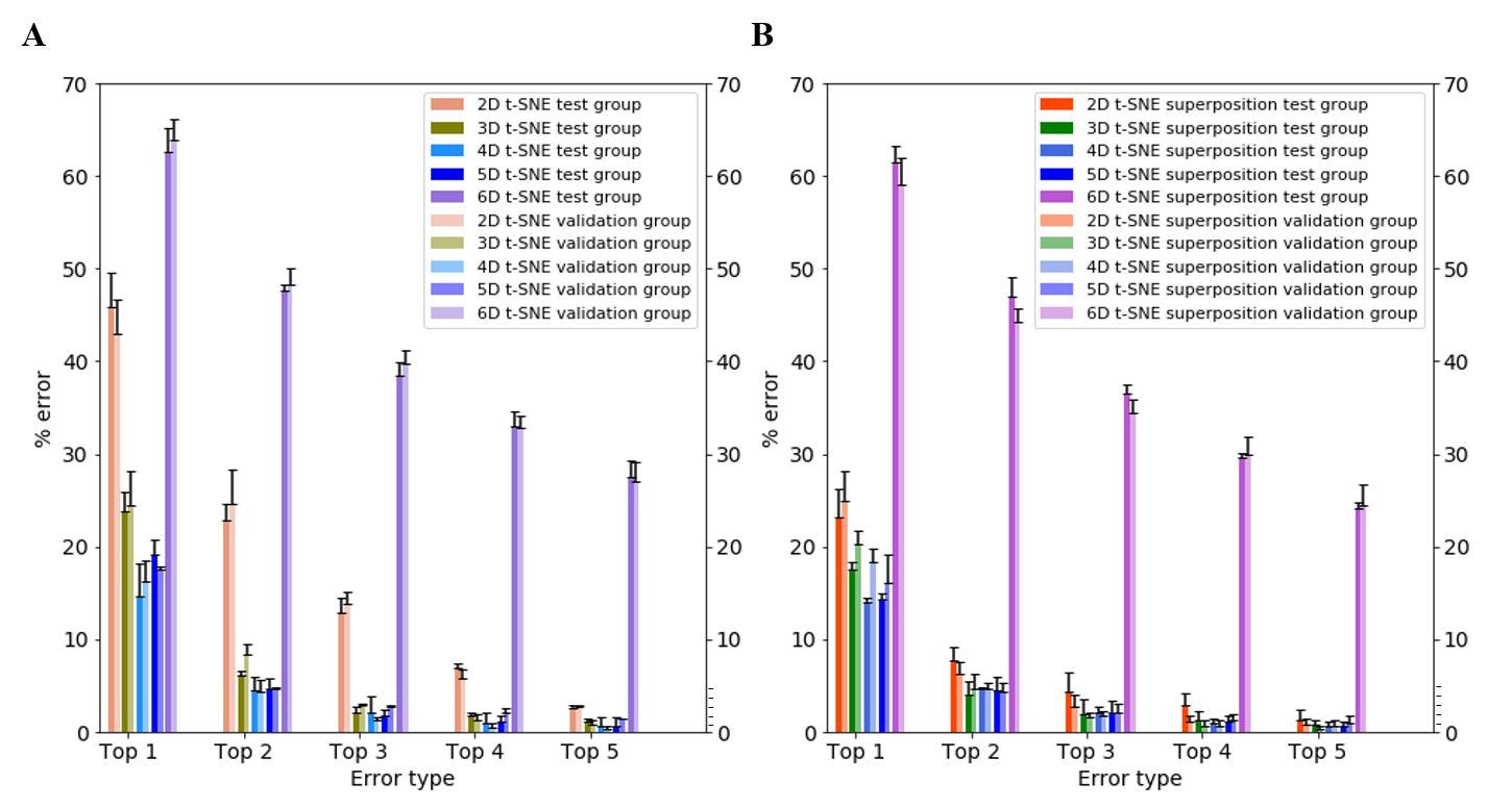
Figure 5. Top-1 through top-5 error scores for 2D, 3D, 4D, 5D and 6D t-SNE. (A) Without superposition. (B) With superposition. Bars represent the average of n = 3 passes of testing sets in the neural net; each testing set is randomized and contains 375 individuals. Error bars represent standard deviation.
These results show that it is possible to significantly improve the accuracy of neural net classification using inputs with certain dimension and/or superposition adjustments. Overall, my neural net’s top-5 error rate is <0.5% for 4D t-SNE, suggesting that the net nearly always predicts the individuals’ self-described label within its first five predictions, with comparable results at top-4 (Figure 5). For comparison, AlexNet, the prototypical neural net that led to the current revolution of neural nets in multiple fields, had a top-5 error of ~17% (Krizhevsky, et al., 2012). I ascribe the high performance of my net to a combination of its architecture, the well-chosen unsupervised dimensional reduction method, and initial processing techniques applied to the WGS datasets.
Discussion:
Machine learning and dimensional reduction techniques are well-suited for the study of high- dimensional datasets. In this study, I demonstrated that multi-dimensional unsupervised t-SNE followed by a neural network can be used for sub-continental genetic ancestry classification of individuals in the 1000 Genomes Project dataset with outstanding accuracy. Additionally, superposition can dramatically improve the neural net classification at lower dimensions such as 2D and 3D, suggesting that neural net architectures that better account for important spatial relationships between objects (e.g., capsule nets (Hinton, et al., 2018; Sabour, et al., 2017)) could be successfully implemented in the future. In addition, I generated contour plots that give mechanistic insight on how my neural nets performed classifications. Being able to see inside the inner workings of these neural nets will lead to further optimizations to stratify populations that were previously thought to be singular into multiple strata (i.e., Japan). Unearthing new populations is interesting in and of itself, but importantly this same work is an essential step towards understanding the genetic background of patients with inherited diseases. Proper stratification removes confounding noise in genetic analyses thus enabling precision medicine causal disease gene identification and gene therapy.
References and Notes:
Bridges, M., et al. Genetic classification of populations using supervised learning. PLoS One 2011;6(5):e14802.
Chang, C.C., et al. Second-generation PLINK: rising to the challenge of larger and richer datasets.
GigaScience 2015;4(1):1-16.
Danecek, P., et al. The variant call format and VCFtools. Bioinformatics 2011;27(15):2156-2158. Genomes Project, C., et al. A global reference for human genetic variation. Nature 2015;526(7571):68- 74.
Haasl, R.J., McCarty, C.A. and Payseur, B.A. Genetic ancestry inference using support vector machines, and the active emergence of a unique American population. Eur J Hum Genet 2013;21(5):554-562.
He, K., et al. Deep Residual Learning for Image Recognition. CoRR 2015;abs/1512.03385. Hellenthal, G., et al. A genetic atlas of human admixture history. Science 2014;343(6172):747-751.
Hinton, G., Sabour, S. and Frosst, N. Matrix Capsules with EM Routing. Conference Paper at ICLR 2018.
Jolliffe, I.T. Principal Component Analysis. New York: Springer-Verlag New York, Inc.; 2002.
Kaplanis, J., et al. Quantitative analysis of population-scale family trees with millions of relatives. Science 2018.
Kaul, P., et al. Genomic ancestry inference with deep learning. Google Cloud Platform Blog https://cloud.google.com/blog/big-data/2017/09/genomic-ancestry-inference-with-deep-learning 2017. Krizhevsky, A., Sutskever, I. and Hinton, G.E. ImageNet Classification with Deep Convolutional Neural Networks. Advances in Neural Information Processing Systems (NIPS 2012) 2012;25.
Manichaikul, A., et al. Robust relationship inference in genome-wide association studies. Bioinformatics 2010;26(22):2867-2873.
Olah, C. Visualizing Representations: Deep Learning and Human Beings. Blog https://colah.github.io/posts/2015-01-Visualizing-Representations/ 2015.
Omberg, L., et al. Inferring genome-wide patterns of admixture in Qataris using fifty-five ancestral populations. BMC Genet 2012;13:49-58.
Pedregosa, F., et al. Scikit-learn: Machine Learning in Python. Journal of Machine Learning Research 2011;12:2825-2830.
Romero, A., et al. Diet Networks: Thin Parameters for Fat Genomics. ICLR 2017:arXiv:1611.09340v09343. Roweis, S.T. and Saul, L.K. Nonlinear Dimensionality Reduction by Locally Linear Embedding. Science 2000;290(5500):2323-2326.
Sabour, S., Frosst, N. and Hinton, G. Dynamic Routing Between Capsules. 31st Conference on Neural Information Processing Systems (NIPS 2017) 2017.
Sammon, J.W. A Nonlinear Mapping for Data Structure Analysis. IEEE Transactions on Computers 1969;C- 18(5):401-409.
Szegedy, C., et al. Going deeper with convolutions. In, 2015 IEEE Conference on Computer Vision and Pattern Recognition (CVPR). 2015. p. 1-9.
Tenenbaum, J.B., de Silva, V. and Langford, J.C. A global geometric framework for nonlinear dimensionality reduction. Science 2000;290(5500):2319-2323.
Tian, C., Gregersen, P.K. and Seldin, M.F. Accounting for ancestry: population substructure and genome- wide association studies. Hum Mol Genet 2008;17(R2):R143-150.
Torgerson, W.S. Multidimensional scaling: I. Theory and method. Psychometrika 1952;17(4):401-419. van der Maaten, L. and Hinton, G. Visualizing Data using t-SNE. Journal of Machine Learning Research 2008;9:2579-2605.
Acknowledgments: The author would like to thank Dr. Greg Jensen for advice on choice of programming languages and Dr. Martin Chalfie for his guidance on fundamental genetics.
Funding: This project was made possible with a startup computational package from Amazon Web Services.
Author contributions: Concepts, Experiments and Manuscript by eMalick G. Njie.
Data and materials availability: All whole genome data used here are publicly available from the 1000 Genomes Project phase III repository ftp://ftp.1000genomes.ebi.ac.uk/vol1/ftp/phase3/ data. t-SNE and Scikit-learn neural network implementations and contour plots are available online in the Scikit-learn python library http://scikit-learn.org. The Lasagne neural net framework is available at https://github.com/Lasagne/Lasagne.
Materials and Methods (For online publication)
General approach
t-SNE was first applied on a hyper-dense, high-dimensional genetic representation of each individual’s WGS dataset. Following t-SNE dimensional reduction, the resultant lower dimensional coordinates (e.g., 3D) of each data point were fed into a neural network for training. The trained neural net was subsequently used to classify individuals according to each of the 26 world populations sampled in the 1000 Genomes Project (Genomes Project, et al., 2015).
Genomic data and preparation
WGS data were obtained from the 1000 Genomes Project phase 3 repository (Genomes Project, et al., 2015). These consist of DNA sequences of 2,504 individuals sampled from 26 populations (heritages) from around the world that were chosen to represent global diversity. A list of the three-letter heritage abbreviations used in this study are as follows: ACB (African Caribbeans in Barbados), ASW (Americans of African Ancestry in SW USA), BEB (Bengali from Bangladesh), CDX (Chinese Dai in Xishuangbanna, China), CEU (Utah Residents (CEPH) with Northern and Western European Ancestry), CHB (Han Chinese in Bejing, China), CHS Southern Han Chinese, CLM (Colombians from Medellin, Colombia), ESN (Esan in Nigeria), FIN (Finnish in Finland), GBR (British in England and Scotland), GIH (Gujarati Indian from Houston, Texas), GWD (Gambian in Western Divisions in the Gambia), IBS (Iberian Population in Spain), ITU (Indian Telugu from the UK), JPT (Japanese in Tokyo, Japan), KHV (Kinh in Ho Chi Minh City, Vietnam), LWK (Luhya in Webuye, Kenya), MSL (Mende in Sierra Leone), MXL (Mexican Ancestry from Los Angeles USA), PEL (Peruvians from Lima, Peru), PJL (Punjabi from Lahore, Pakistan), PUR (Puerto Ricans from Puerto Rico), STU (Sri Lankan Tamil from the UK), TSI (Toscani in Italia), YRI (Yoruba in Ibadan, Nigeria) (Genomes Project, et al., 2015).
To conserve processing and storage resources, I limited my examination to chromosome 1 variations from the GRCh37 reference genome. These variations were represented in Variant Call Format (VCF) files (Danecek, et al., 2011) and converted to bed files using pLink2 (Chang, et al., 2015). These bed files have hyper dense chromosomal representations of ~6 million SNPs and include all regions (i.e., exons and non-coding regions). The bed files were input into KING (Manichaikul, et al., 2010) to obtain pairwise coefficients of the relatedness of each individual to every other member of the set. A matrix composed of these KING coefficients was generated and used as input into t-SNE.
Non-linear dimensional reduction using t-SNE
The unsupervised non-linear dimensional reduction technique t-SNE (Scikit-learn implementation) was applied (Pedregosa, et al., 2011; van der Maaten and Hinton, 2008). Unless otherwise stated, the parameters adopted were: perplexity = 30, learning rate = 200, and early exaggeration = 12 for 1000 iterations. Various number of output dimensions (i.e., 2D to 6D) were tested. For superposition, one additional t-SNE frame was used as an input into the neural net. This second input frame was generated at perplexity = 40, while keeping all other parameters constant.
Ancestry classification using a neural network
The output of t-SNE (i.e., the Cartesian coordinates of each individual in t-SNE space) was split into randomized training, testing, and validation sets. The training set was used for supervised learning of the neural network. Analyses of classification was performed on the testing set and verified on the validation set. Unless otherwise stated, the neural network was comprised of a Theano-based stack with nolearn layered atp 5-layered Lasagna, including non- linear ReLU activations and a SoftMax output layer. The input layer consisted of 2, 3, 4, 5 or 6 neurons for 2D, 3D, 4D, 5D or 6D t-SNE respectively (i.e., 2 neurons for x and y, 3 for x, y, and z, and so forth). For superposition, two frames of t-SNE were used as input into the neural net.
Thus, the number of input neurons were doubled to 4, 6, 8, 10 or 12 neurons for 2D, 3D, 4D, 5D or 6D t-SNE, respectively. The input layer was followed by 3 hidden layers composed of a dense layer of 500 neurons, a 50% dropout layer of 500 neurons, and a dense layer of 100 hidden neurons. This structure terminated in a final output layer of 26 neurons, each sensitive to a single heritage from the 26 world populations in the 1000 Genomes Project dataset (Genomes Project, et al., 2015). Regularization was achieved mainly by dropout. Software was written in python within iPython interactive development environments.